Plot Functions¶

This module has functions that allows us to create charts that helps us to analyze quickly the properties of our optimal portfolios.

The following example construct the portfolios and the efficient frontier that will be plot using the functions of this module.

Example¶

import numpy as np
import pandas as pd
import yfinance as yf
import riskfolio as rp

# Date range
start = '2016-01-01'
end = '2019-12-30'

# Tickers of assets
assets = ['JCI', 'TGT', 'CMCSA', 'CPB', 'MO', 'APA', 'MRSH', 'JPM',
          'ZION', 'PSA', 'BAX', 'BMY', 'LUV', 'PCAR', 'TXT', 'TMO',
          'DE', 'MSFT', 'HPQ', 'SEE', 'VZ', 'CNP', 'NI', 'T', 'BA']
assets.sort()

# Tickers of factors
factors = ['MTUM', 'QUAL', 'VLUE', 'SIZE', 'USMV']
factors.sort()

tickers = assets + factors
tickers.sort()

# Downloading the data
data = yf.download(tickers, start = start, end = end)
data = data.loc[:,('Adj Close', slice(None))]
data.columns = tickers
returns = data.pct_change().dropna()

Y = returns[assets]
X = returns[factors]

# Creating the Portfolio Object
port = rp.Portfolio(returns=Y)

# To display dataframes values in percentage format
pd.options.display.float_format = '{:.4%}'.format

# Choose the risk measure
rm = 'MSV'  # Semi Standard Deviation

# Estimate inputs of the model (historical estimates)
method_mu='hist' # Method to estimate expected returns based on historical data.
method_cov='hist' # Method to estimate covariance matrix based on historical data.

port.assets_stats(method_mu=method_mu, method_cov=method_cov)

mu = port.mu
cov = port.cov

# Estimate the portfolio that maximizes the risk adjusted return ratio
w1 = port.optimization(model='Classic', rm=rm, obj='Sharpe', rf=0.0, l=0, hist=True)

# Estimate points in the efficient frontier mean - semi standard deviation
ws = port.efficient_frontier(model='Classic', rm=rm, points=20, rf=0, hist=True)

# Estimate the risk parity portfolio for semi standard deviation
w2 = port.rp_optimization(model='Classic', rm=rm, rf=0, b=None, hist=True)

# Estimate the risk parity portfolio for semi standard deviation
w2 = port.rp_optimization(model='Classic', rm=rm, rf=0, b=None, hist=True)

# Estimate the risk parity portfolio for risk factors
port.factors = X
port.factors_stats(method_mu=method_mu,
                   method_cov=method_cov,
                   feature_selection='stepwise',
                   stepwise='Forward')
w3 = port.rp_optimization(model='FC', rm='MV', rf=0, b_f=None)

# Estimate the risk parity portfolio for principal components
port.factors = X
port.factors_stats(method_mu=method_mu,
                   method_cov=method_cov,
                   feature_selection='PCR',
                   n_components=0.95)
w4 = port.rp_optimization(model='FC', rm='MV', rf=0, b_f=None)

wb = pd.DataFrame(np.ones((len(assets), 1))/len(assets), index=assets)

Module Functions¶

PlotFunctions.plot_series(returns, w, cmap='tab20', n_colors=20, height=6, width=10, ax=None)[source]¶

Create a chart with the compounded cumulative of the portfolios.

Parameters:¶

returns : DataFrame of shape (n_samples, n_assets)¶: Assets returns DataFrame, where n_samples is the number of observations and n_assets is the number of assets.
w : DataFrame or Series of shape (n_assets, 1)¶: Portfolio weights, where n_assets is the number of assets.
cmap : cmap, optional¶: Colorscale used to plot each portfolio compounded cumulative return. The default is ‘tab20’.
n_colors : int, optional¶: Number of distinct colors per color cycle. If there are more assets than n_colors, the chart is going to start to repeat the color cycle. The default is 20.
height : float, optional¶: Height of the image in inches. The default is 6.
width : float, optional¶: Width of the image in inches. The default is 10.
ax : matplotlib axis, optional¶: If provided, plot on this axis. The default is None.

Raises:¶

ValueError – When the value cannot be calculated.

Returns:¶

ax – Returns the Axes object with the plot for further tweaking.

Return type:¶

matplotlib axis

Example

ax = rp.plot_series(returns=Y,
                    w=ws,
                    cmap='tab20',
                    height=6,
                    width=10,
                    ax=None)

PlotFunctions.plot_frontier(w_frontier, returns, mu=None, cov=None, rm='MV', kelly=False, rf=0, alpha=0.05, a_sim=100, beta=None, b_sim=None, kappa=0.3, kappa_g=None, p_em=2, p_esm=2, solver='CLARABEL', cmap='viridis', w=None, label='Portfolio', marker='*', s=16, c='r', height=6, width=10, t_factor=252, ax=None)[source]¶

Creates a plot of the efficient frontier for a risk measure specified by the user.

Parameters:¶

w_frontier : DataFrame¶

Portfolio weights of some points in the efficient frontier.

mu : DataFrame of shape (1, n_assets)¶

Vector of expected returns, where n_assets is the number of assets.

cov : DataFrame of shape (n_assets, n_assets)¶

Covariance matrix, where n_assets is the number of assets.

returns : DataFrame of shape (n_samples, n_assets)¶

Assets returns DataFrame, where n_samples is the number of observations and n_assets is the number of assets.

rm : str, optional¶

The risk measure used to estimate the frontier. The default is ‘MV’. Possible values are:

’MV’: Standard Deviation.
’KT’: Square Root Kurtosis.
’EM’: p_em Root of Even Moment or order 2 * p_em.
’MAD’: Mean Absolute Deviation.
’GMD’: Gini Mean Difference.
’MSV’: Semi Standard Deviation.
’SKT’: Square Root Semi Kurtosis.
’ESM’: p_esm Root of Even Semi Moment or order 2 * p_esm.
’FLPM’: First Lower Partial Moment (Omega Ratio).
’SLPM’: Second Lower Partial Moment (Sortino Ratio).
’CVaR’: Conditional Value at Risk.
’TG’: Tail Gini.
’EVaR’: Entropic Value at Risk.
’RLVaR’: Relativistic Value at Risk.
’WR’: Worst Realization (Minimax).
’CVRG’: CVaR range of returns.
’TGRG’: Tail Gini range of returns.
’EVRG’: EVaR range of returns.
’RVRG’: RLVaR range of returns.
’RG’: Range of returns.
’MDD’: Maximum Drawdown of uncompounded returns (Calmar Ratio).
’ADD’: Average Drawdown of uncompounded cumulative returns.
’CDaR’: Conditional Drawdown at Risk of uncompounded cumulative returns.
’EDaR’: Entropic Drawdown at Risk of uncompounded cumulative returns.
’RLDaR’: Relativistic Drawdown at Risk of uncompounded cumulative returns.
’UCI’: Ulcer Index of uncompounded cumulative returns.

kelly : bool, optional¶

Method used to calculate mean return. Possible values are False for arithmetic mean return and True for mean logarithmic return. The default is False.

rf : float, optional¶

Risk free rate or minimum acceptable return. The default is 0.

alpha : float, optional¶

Significance level of VaR, CVaR, EVaR, RLVaR, DaR, CDaR, EDaR, RLDaR and Tail Gini of losses. The default is 0.05.

a_sim : float, optional¶

Number of CVaRs used to approximate Tail Gini of losses. The default is 100.

beta : float, optional¶

Significance level of CVaR and Tail Gini of gains. If None it duplicates alpha value. The default is None.

b_sim : float, optional¶

Number of CVaRs used to approximate Tail Gini of gains. If None it duplicates a_sim value. The default is None.

kappa : float, optional¶

Deformation parameter of RLVaR and RLDaR for losses, must be between 0 and 1. The default is 0.30.

kappa_g : float, optional¶

Deformation parameter of RLVaR for gains, must be between 0 and 1. The default is None.

p_em : int, optional¶

Order of the Even Moment of order 2 * p_em. It must be an integer higher equal than 2. The default value is 2.

p_esm : int, optional¶

Order of the Even Semi Moment of order 2 * p_esm. It must be an integer higher equal than 2. The default value is 2.

solver : str, optional¶

Solver available for CVXPY that supports power cone programming. Used to calculate RLVaR and RLDaR. The default value is ‘CLARABEL’.

cmap : cmap, optional¶

Colorscale that represents the risk adjusted return ratio. The default is ‘viridis’.

w : DataFrame or Series of shape (n_assets, 1), optional¶

A portfolio specified by the user. The default is None.

label : str or list, optional¶

Name or list of names of portfolios that appear on plot legend. The default is ‘Portfolio’.

marker : str, optional¶

Marker of w. The default is “*”.

s : float, optional¶

Size of marker. The default is 16.

c : str, optional¶

Color of marker. The default is ‘r’.

height : float, optional¶

Height of the image in inches. The default is 6.

width : float, optional¶

Width of the image in inches. The default is 10.

t_factor : float, optional¶

Factor used to annualize expected return and expected risks for risk measures based on returns (not drawdowns). The default is 252.

\[\begin{split}\begin{align} \text{Annualized Return} & = \text{Return} \, \times \, \text{t_factor} \\ \text{Annualized Risk} & = \text{Risk} \, \times \, \sqrt{\text{t_factor}} \end{align}\end{split}\]

ax : matplotlib axis, optional¶

If provided, plot on this axis. The default is None.

Raises:¶

ValueError – When the value cannot be calculated.

Returns:¶

ax – Returns the Axes object with the plot for further tweaking.

Return type:¶

matplotlib Axes

Example

label = 'Max Risk Adjusted Return Portfolio'
mu = port.mu
cov = port.cov
returns = port.returns

ax = rp.plot_frontier(w_frontier=ws,
                      mu=mu,
                      cov=cov,
                      returns=Y,
                      rm=rm,
                      rf=0,
                      alpha=0.05,
                      cmap='viridis',
                      w=w1,
                      label=label,
                      marker='*',
                      s=16,
                      c='r',
                      height=6,
                      width=10,
                      t_factor=252,
                      ax=None)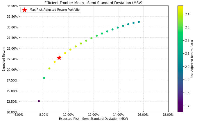

PlotFunctions.plot_pie(w, title='', others=0.05, nrow=25, cmap='tab20', n_colors=20, height=6, width=8, ax=None)[source]¶

Create a pie chart with portfolio weights.

Parameters:¶

w : DataFrame or Series of shape (n_assets, 1)¶: Portfolio weights, where n_assets is the number of assets.
title : str, optional¶: Title of the chart. The default is “”.
others : float, optional¶: Percentage of others section. The default is 0.05.
nrow : int, optional¶: Number of rows of the legend. The default is 25.
cmap : cmap, optional¶: Color scale used to plot each asset weight. The default is ‘tab20’.
n_colors : int, optional¶: Number of distinct colors per color cycle. If there are more assets than n_colors, the chart is going to start to repeat the color cycle. The default is 20.
height : float, optional¶: Height of the image in inches. The default is 10.
width : float, optional¶: Width of the image in inches. The default is 10.
ax : matplotlib axis, optional¶: If provided, plot on this axis. The default is None.

Raises:¶

ValueError – When the value cannot be calculated.

Returns:¶

ax – Returns the Axes object with the plot for further tweaking.

Return type:¶

matplotlib axis.

Example

ax = rp.plot_pie(w=w1,
                 title='Portfolio',
                 height=6,
                 width=10,
                 cmap="tab20",
                 ax=None)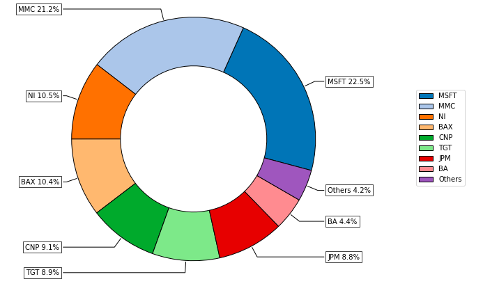

PlotFunctions.plot_bar(w, title='', kind='v', others=0.05, nrow=25, cpos='tab:green', cneg='darkorange', cothers='dodgerblue', height=6, width=10, ax=None)[source]¶

Create a bar chart with portfolio weights.

Parameters:¶

w : DataFrame or Series of shape (n_assets, 1)¶: Portfolio weights, where n_assets is the number of assets.
title : str, optional¶: Title of the chart. The default is “”.
kind : str, optional¶: Kind of bar plot, “v” for vertical bars and “h” for horizontal bars. The default is “v”.
others : float, optional¶: Percentage of others section. The default is 0.05.
nrow : int, optional¶: Max number of bars that be plotted. The default is 25.
cpos : str, optional¶: Color for positives weights. The default is ‘tab:green’.
cneg : str, optional¶: Color for negatives weights. The default is ‘darkorange’.
cothers : str, optional¶: Color for others bar. The default is ‘dodgerblue’.
height : float, optional¶: Height of the image in inches. The default is 10.
width : float, optional¶: Width of the image in inches. The default is 10.
ax : matplotlib axis, optional¶: If provided, plot on this axis. The default is None.

Raises:¶

ValueError – When the value cannot be calculated.

Returns:¶

ax – Returns the Axes object with the plot for further tweaking.

Return type:¶

matplotlib axis.

Example

ax = rp.plot_bar(w1,
                 title='Portfolio',
                 kind="v",
                 others=0.05,
                 nrow=25,
                 height=6,
                 width=10,
                 ax=None)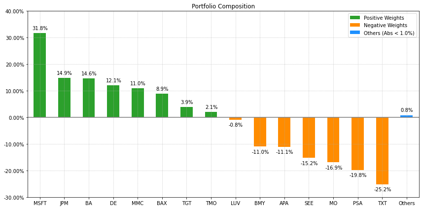

PlotFunctions.plot_frontier_area(w_frontier, nrow=25, cmap='tab20', n_colors=20, height=6, width=10, ax=None)[source]¶

Create a chart with the asset composition of the efficient frontier.

Parameters:¶

w_frontier : DataFrame¶: Weights of portfolios in the efficient frontier.
nrow : int, optional¶: Number of rows of the legend. The default is 25.
cmap : cmap, optional¶: Color scale used to plot each asset weight. The default is ‘tab20’.
n_colors : int, optional¶: Number of distinct colors per color cycle. If there are more assets than n_colors, the chart is going to start to repeat the color cycle. The default is 20.
height : float, optional¶: Height of the image in inches. The default is 6.
width : float, optional¶: Width of the image in inches. The default is 10.
ax : matplotlib axis, optional¶: If provided, plot on this axis. The default is None.

Raises:¶

ValueError – When the value cannot be calculated.

Returns:¶

ax – Returns the Axes object with the plot for further tweaking.

Return type:¶

matplotlib axis.

Example

ax = rp.plot_frontier_area(w_frontier=ws,
                           cmap="tab20",
                           height=6,
                           width=10,
                           ax=None)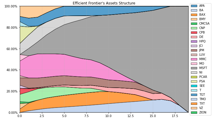

PlotFunctions.plot_risk_con(w, returns, cov=None, asset_classes=None, classes_col=None, rm='MV', rf=0, alpha=0.05, a_sim=100, beta=None, b_sim=None, kappa=0.3, kappa_g=None, p_em=2, p_esm=2, solver='CLARABEL', percentage=False, erc_line=True, color='tab:blue', erc_linecolor='r', height=6, width=10, t_factor=252, ax=None)[source]¶

Create a chart with the risk contribution per asset of the portfolio.

Parameters:¶

w : DataFrame or Series of shape (n_assets, 1)¶

Portfolio weights, where n_assets is the number of assets.

returns : DataFrame of shape (n_samples, n_assets)¶

Assets returns DataFrame, where n_samples is the number of observations and n_assets is the number of assets.

cov : DataFrame of shape (n_assets, n_assets)¶

Covariance matrix, where n_assets is the number of assets.

asset_classes : DataFrame of shape (n_assets, n_cols)¶

Asset’s classes DataFrame, where n_assets is the number of assets and n_cols is the number of columns of the DataFrame where the first column is the asset list and the next columns are the different asset’s classes sets. It is only used when kind value is ‘classes’. The default value is None.

classes_col : str or int¶

If value is str, it is the column name of the set of classes from asset_classes dataframe. If value is int, it is the column number of the set of classes from asset_classes dataframe. The default value is None.

rm : str, optional¶

Risk measure used to estimate risk contribution. The default is ‘MV’. Possible values are:

’MV’: Standard Deviation.
’KT’: Square Root Kurtosis.
’EM’: p_em Root of Even Moment of Order 2 * p_em.
’MAD’: Mean Absolute Deviation.
’GMD’: Gini Mean Difference.
’MSV’: Semi Standard Deviation.
’SKT’: Square Root Semi Kurtosis.
’ESM’: p_esm Root of Even Semi Moment of Order 2 * p_esm.
’FLPM’: First Lower Partial Moment (Omega Ratio).
’SLPM’: Second Lower Partial Moment (Sortino Ratio).
’CVaR’: Conditional Value at Risk.
’TG’: Tail Gini.
’EVaR’: Entropic Value at Risk.
’RLVaR’: Relativistic Value at Risk.
’WR’: Worst Realization (Minimax).
’CVRG’: CVaR range of returns.
’TGRG’: Tail Gini range of returns.
’EVRG’: EVaR range of returns.
’RVRG’: RLVaR range of returns.
’RG’: Range of returns.
’MDD’: Maximum Drawdown of uncompounded cumulative returns (Calmar Ratio).
’ADD’: Average Drawdown of uncompounded cumulative returns.
’CDaR’: Conditional Drawdown at Risk of uncompounded cumulative returns.
’EDaR’: Entropic Drawdown at Risk of uncompounded cumulative returns.
’RLDaR’: Relativistic Drawdown at Risk of uncompounded cumulative returns.
’UCI’: Ulcer Index of uncompounded cumulative returns.

rf : float, optional¶

Risk free rate or minimum acceptable return. The default is 0.

alpha : float, optional¶

Significance level of VaR, CVaR, Tail Gini, EVaR, RLVaR, CDaR, EDaR and RLDaR. The default is 0.05.

a_sim : float, optional¶

Number of CVaRs used to approximate Tail Gini of losses. The default is 100.

beta : float, optional¶

Significance level of CVaR and Tail Gini of gains. If None it duplicates alpha value. The default is None.

b_sim : float, optional¶

Number of CVaRs used to approximate Tail Gini of gains. If None it duplicates a_sim value. The default is None.

kappa : float, optional¶

Deformation parameter of RLVaR and RLDaR for losses, must be between 0 and 1. The default is 0.30.

kappa_g : float, optional¶

Deformation parameter of RLVaR for gains, must be between 0 and 1. The default is None.

p_em : int, optional¶

Order of the Even Moment of order 2 * p_em. It must be an integer higher equal than 2. The default value is 2.

p_esm : int, optional¶

Order of the Even Semi Moment of order 2 * p_esm. It must be an integer higher equal than 2. The default value is 2.

solver : str, optional¶

Solver available for CVXPY that supports power cone programming. Used to calculate RLVaR and RLDaR. The default value is ‘CLARABEL’.

percentage : bool, optional¶

If risk contribution per asset is expressed as percentage or as a value. The default is False.

erc_line : bool, optional¶

If equal risk contribution line is plotted. The default is False.

color : str, optional¶

Color used to plot each asset risk contribution. The default is ‘tab:blue’.

erc_linecolor : str, optional¶

Color used to plot equal risk contribution line. The default is ‘r’.

height : float, optional¶

Height of the image in inches. The default is 6.

width : float, optional¶

Width of the image in inches. The default is 10.

t_factor : float, optional¶

Factor used to annualize expected return and expected risks for risk measures based on returns (not drawdowns). The default is 252.

ax : matplotlib axis, optional¶

If provided, plot on this axis. The default is None.

Raises:¶

ValueError – When the value cannot be calculated.

Returns:¶

ax – Returns the Axes object with the plot for further tweaking.

Return type:¶

matplotlib axis.

Example

ax = rp.plot_risk_con(w=w2,
                      cov=cov,
                      returns=Y,
                      rm=rm,
                      rf=0,
                      alpha=0.05,
                      color="tab:blue",
                      height=6,
                      width=10,
                      t_factor=252,
                      ax=None)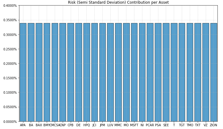

PlotFunctions.plot_factor_risk_con(w, returns, factors, cov=None, B=None, const=True, rm='MV', rf=0, alpha=0.05, a_sim=100, beta=None, b_sim=None, kappa=0.3, kappa_g=None, p_em=2, p_esm=2, solver='CLARABEL', feature_selection='stepwise', stepwise='Forward', criterion='pvalue', threshold=0.05, n_components=0.95, percentage=False, erc_line=True, color='tab:orange', erc_linecolor='r', height=6, width=10, t_factor=252, ax=None)[source]¶

Create a chart with the risk contribution per risk factor of the portfolio.

Parameters:¶

w : DataFrame or Series of shape (n_assets, 1)¶

Portfolio weights, where n_assets is the number of assets.

cov : DataFrame of shape (n_assets, n_assets)¶

Covariance matrix, where n_assets is the number of assets.

returns : DataFrame of shape (n_samples, n_assets)¶

Assets returns DataFrame, where n_samples is the number of observations and n_assets is the number of assets.

factors : DataFrame or nd-array of shape (n_samples, n_factors)¶

Risk factors returns DataFrame, where n_samples is the number of samples and n_factors is the number of factors.

B : DataFrame of shape (n_assets, n_factors), optional¶

Loadings matrix, where n_assets is the number assets and n_factors is the number of risk factors. If is not specified, is estimated using stepwise regression. The default is None.

const : bool, optional¶

Indicate if the loadings matrix has a constant. The default is False.

rm : str, optional¶

Risk measure used to estimate risk contribution. The default is ‘MV’. Possible values are:

’MV’: Standard Deviation.
’KT’: Square Root Kurtosis.
’EM’: p_em Root of Even Moment of Order 2 * p_em.
’MAD’: Mean Absolute Deviation.
’GMD’: Gini Mean Difference.
’MSV’: Semi Standard Deviation.
’SKT’: Square Root Semi Kurtosis.
’ESM’: p_esm Root of Even Semi Moment of Order 2 * p_esm.
’FLPM’: First Lower Partial Moment (Omega Ratio).
’SLPM’: Second Lower Partial Moment (Sortino Ratio).
’CVaR’: Conditional Value at Risk.
’TG’: Tail Gini.
’EVaR’: Entropic Value at Risk.
’RLVaR’: Relativistic Value at Risk.
’WR’: Worst Realization (Minimax).
’CVRG’: CVaR range of returns.
’TGRG’: Tail Gini range of returns.
’EVRG’: EVaR range of returns.
’RVRG’: RLVaR range of returns.
’RG’: Range of returns.
’MDD’: Maximum Drawdown of uncompounded cumulative returns (Calmar Ratio).
’ADD’: Average Drawdown of uncompounded cumulative returns.
’CDaR’: Conditional Drawdown at Risk of uncompounded cumulative returns.
’EDaR’: Entropic Drawdown at Risk of uncompounded cumulative returns.
’RLDaR’: Relativistic Drawdown at Risk of uncompounded cumulative returns.
’UCI’: Ulcer Index of uncompounded cumulative returns.

rf : float, optional¶

Risk free rate or minimum acceptable return. The default is 0.

alpha : float, optional¶

Significance level of VaR, CVaR, Tail Gini, EVaR, RLVaR, CDaR, EDaR and RLDaR. The default is 0.05.

a_sim : float, optional¶

Number of CVaRs used to approximate Tail Gini of losses. The default is 100.

beta : float, optional¶

Significance level of CVaR and Tail Gini of gains. If None it duplicates alpha value. The default is None.

b_sim : float, optional¶

Number of CVaRs used to approximate Tail Gini of gains. If None it duplicates a_sim value. The default is None.

kappa : float, optional¶

Deformation parameter of RLVaR and RLDaR for losses, must be between 0 and 1. The default is 0.30.

kappa_g : float, optional¶

Deformation parameter of RLVaR for gains, must be between 0 and 1. The default is None.

p_em : int, optional¶

Order of the Even Moment of order 2 * p_em. It must be an integer higher equal than 2. The default value is 2.

p_esm : int, optional¶

Order of the Even Semi Moment of order 2 * p_esm. It must be an integer higher equal than 2. The default value is 2.

solver : str, optional¶

Solver available for CVXPY that supports power cone programming. Used to calculate RLVaR and RLDaR. The default value is ‘CLARABEL’.

feature_selection : str 'stepwise' or 'PCR', optional¶

Indicate the method used to estimate the loadings matrix. The default is ‘stepwise’.

stepwise : str 'Forward' or 'Backward', optional¶

Indicate the method used for stepwise regression. The default is ‘Forward’.

criterion : str, optional¶

The default is ‘pvalue’. Possible values of the criterion used to select the best features are:

’pvalue’: select the features based on p-values.
’AIC’: select the features based on lowest Akaike Information Criterion.
’SIC’: select the features based on lowest Schwarz Information Criterion.
’R2’: select the features based on highest R Squared.
’R2_A’: select the features based on highest Adjusted R Squared.

threshold : scalar, optional¶

Is the maximum p-value for each variable that will be accepted in the model. The default is 0.05.

n_components : int, float, None or str, optional¶

if 1 < n_components (int), it represents the number of components that will be keep. if 0 < n_components < 1 (float), it represents the percentage of variance that the is explained by the components kept. See PCA for more details. The default is 0.95.

percentage : bool, optional¶

If risk contribution per asset is expressed as percentage or as a value. The default is False.

erc_line : bool, optional¶

If equal risk contribution line is plotted. The default is False.

color : str, optional¶

Color used to plot each asset risk contribution. The default is ‘tab:orange’.

erc_linecolor : str, optional¶

Color used to plot equal risk contribution line. The default is ‘r’.

height : float, optional¶

Height of the image in inches. The default is 6.

width : float, optional¶

Width of the image in inches. The default is 10.

t_factor : float, optional¶

Factor used to annualize expected return and expected risks for risk measures based on returns (not drawdowns). The default is 252.

ax : matplotlib axis, optional¶

If provided, plot on this axis. The default is None.

Raises:¶

ValueError – When the value cannot be calculated.

Returns:¶

ax – Returns the Axes object with the plot for further tweaking.

Return type:¶

matplotlib axis.

Example

ax = rp.plot_factor_risk_con(w=w3,
                             cov=cov,
                             returns=Y,
                             factors=X,
                             B=None,
                             const=True,
                             rm=rm,
                             rf=0,
                             feature_selection="stepwise",
                             stepwise="Forward",
                             criterion="pvalue",
                             threshold=0.05,
                             height=6,
                             width=10,
                             t_factor=252,
                             ax=None)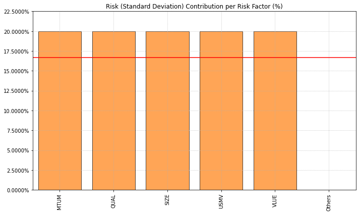

ax = rp.plot_factor_risk_con(w=w4,
                             cov=cov,
                             returns=Y,
                             factors=X,
                             B=None,
                             const=True,
                             rm=rm,
                             rf=0,
                             feature_selection="PCR",
                             n_components=0.95,
                             height=6,
                             width=10,
                             t_factor=252,
                             ax=None)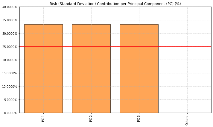

PlotFunctions.plot_hist(returns, w, alpha=0.05, a_sim=100, kappa=0.3, solver='CLARABEL', bins=50, height=6, width=10, ax=None)[source]¶

Create a histogram of portfolio returns with the risk measures.

Parameters:¶

returns : DataFrame of shape (n_samples, n_assets)¶: Assets returns DataFrame, where n_samples is the number of observations and n_assets is the number of assets.
w : DataFrame or Series of shape (n_assets, 1)¶: Portfolio weights, where n_assets is the number of assets.
alpha : float, optional¶: Significance level of VaR, CVaR, EVaR, RLVaR and Tail Gini. The default is 0.05.
a_sim : float, optional¶: Number of CVaRs used to approximate Tail Gini of losses. The default is 100.
kappa : float, optional¶: Deformation parameter of RLVaR and RLDaR, must be between 0 and 1. The default is 0.30.
solver : str, optional¶: Solver available for CVXPY that supports power cone programming. Used to calculate RLVaR and RLDaR. The default value is ‘CLARABEL’.
bins : float, optional¶: Number of bins of the histogram. The default is 50.
height : float, optional¶: Height of the image in inches. The default is 6.
width : float, optional¶: Width of the image in inches. The default is 10.
ax : matplotlib axis, optional¶: If provided, plot on this axis. The default is None.

Raises:¶

ValueError – When the value cannot be calculated.

Returns:¶

ax – Returns the Axes object with the plot for further tweaking.

Return type:¶

matplotlib axis.

Example

ax = rp.plot_hist(returns=Y,
                  w=w1,
                  alpha=0.05,
                  bins=50,
                  height=6,
                  width=10,
                  ax=None)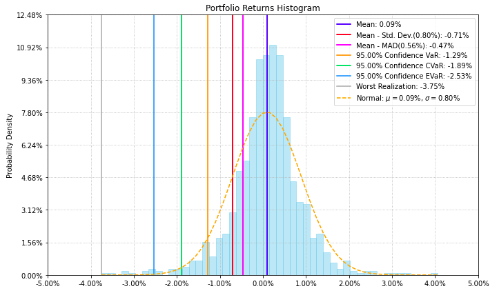

PlotFunctions.plot_range(returns, w, alpha=0.05, a_sim=100, beta=None, b_sim=None, kappa=0.3, kappa_g=0.3, solver='CLARABEL', bins=50, height=6, width=10, ax=None)[source]¶

Create a histogram of portfolio returns with the range risk measures.

Parameters:¶

returns : DataFrame of shape (n_samples, n_assets)¶: Assets returns DataFrame, where n_samples is the number of observations and n_assets is the number of assets.
w : DataFrame or Series of shape (n_assets, 1)¶: Portfolio weights, where n_assets is the number of assets.
alpha : float, optional¶: Significance level of CVaR and Tail Gini of losses. The default is 0.05.
a_sim : float, optional¶: Number of CVaRs used to approximate Tail Gini of losses. The default is 100.
beta : float, optional¶: Significance level of CVaR and Tail Gini of gains. If None it duplicates alpha value. The default is None.
b_sim : float, optional¶: Number of CVaRs used to approximate Tail Gini of gains. If None it duplicates a_sim value. The default is None.
bins : float, optional¶: Number of bins of the histogram. The default is 50.
height : float, optional¶: Height of the image in inches. The default is 6.
width : float, optional¶: Width of the image in inches. The default is 10.
ax : matplotlib axis, optional¶: If provided, plot on this axis. The default is None.

Raises:¶

ValueError – When the value cannot be calculated.

Returns:¶

ax – Returns the Axes object with the plot for further tweaking.

Return type:¶

matplotlib axis.

Example

ax = rp.plot_range(returns=Y,
                   w=w1,
                   alpha=0.05,
                   a_sim=100,
                   beta=None,
                   b_sim=None,
                   bins=50,
                   height=6,
                   width=10,
                   ax=None)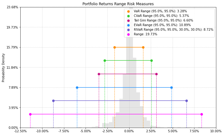

PlotFunctions.plot_drawdown(returns, w, alpha=0.05, kappa=0.3, solver='CLARABEL', height=8, width=10, height_ratios=[2, 3], ax=None)[source]¶

Create a chart with the evolution of portfolio prices and drawdown.

Parameters:¶

returns : DataFrame of shape (n_samples, n_assets)¶: Assets returns DataFrame, where n_samples is the number of observations and n_assets is the number of assets.
w : DataFrame or Series of shape (n_assets, 1)¶: Portfolio weights, where n_assets is the number of assets.
alpha : float, optional¶: Significance level of DaR, CDaR, EDaR and RLDaR. The default is 0.05.
kappa : float, optional¶: Deformation parameter of RLVaR and RLDaR, must be between 0 and 1. The default is 0.30.
solver : str, optional¶: Solver available for CVXPY that supports power cone programming. Used to calculate RLVaR and RLDaR. The default value is ‘CLARABEL’.
height : float, optional¶: Height of the image in inches. The default is 8.
width : float, optional¶: Width of the image in inches. The default is 10.
height_ratios : list or ndarray¶: Defines the relative heights of the rows. Each row gets a relative height of height_ratios[i] / sum(height_ratios). The default value is [2,3].
ax : matplotlib axis of size (2,1), optional¶: If provided, plot on this axis. The default is None.

Raises:¶

ValueError – When the value cannot be calculated.

Returns:¶

ax – Returns the a np.array with Axes objects with plots for further tweaking.

Return type:¶

np.array

Example

ax = rp.plot_drawdown(returns=Y,
                      w=w1,
                      alpha=0.05,
                      height=8,
                      width=10,
                      ax=None)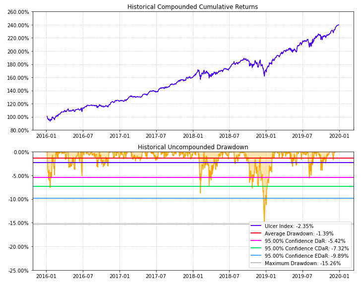

PlotFunctions.plot_table(returns, w, MAR=0, alpha=0.05, a_sim=100, kappa=0.3, solver='CLARABEL', height=9, width=12, t_factor=252, ini_days=1, days_per_year=252, ax=None)[source]¶

Create a table with information about risk measures and risk adjusted return ratios.

Parameters:¶

returns : DataFrame of shape (n_samples, n_assets)¶

Assets returns DataFrame, where n_samples is the number of observations and n_assets is the number of assets.

w : DataFrame or Series of shape (n_assets, 1)¶

Portfolio weights, where n_assets is the number of assets.

MAR : float, optional¶

Minimum acceptable return.

alpha : float, optional¶

Significance level of VaR, CVaR, Tail Gini, EVaR, RLVaR, CDaR, EDaR and RLDaR. The default is 0.05.

a_sim : float, optional¶

Number of CVaRs used to approximate Tail Gini of losses. The default is 100.

kappa : float, optional¶

Deformation parameter of RLVaR and RLDaR, must be between 0 and 1. The default is 0.30.

solver : str, optional¶

Solver available for CVXPY that supports power cone programming. Used to calculate RLVaR and RLDaR. The default value is ‘CLARABEL’.

height : float, optional¶

Height of the image in inches. The default is 9.

width : float, optional¶

Width of the image in inches. The default is 12.

t_factor : float, optional¶

Factor used to annualize expected return and expected risks for risk measures based on returns (not drawdowns). The default is 252.

ini_days : float, optional¶

If provided, it is the number of days of compounding for first return. It is used to calculate Compound Annual Growth Rate (CAGR). This value depend on assumptions used in t_factor, for example if data is monthly you can use 21 (252 days per year) or 30 (360 days per year). The default is 1 for daily returns.

days_per_year : float, optional¶

Days per year assumption. It is used to calculate Compound Annual Growth Rate (CAGR). Default value is 252 trading days per year.

ax : matplotlib axis, optional¶

If provided, plot on this axis. The default is None.

Raises:¶

ValueError – When the value cannot be calculated.

Returns:¶

ax – Returns the Axes object with the plot for further tweaking.

Return type:¶

matplotlib axis

Example

ax = rp.plot_table(returns=Y,
                   w=w1,
                   MAR=0,
                   alpha=0.05,
                   ax=None)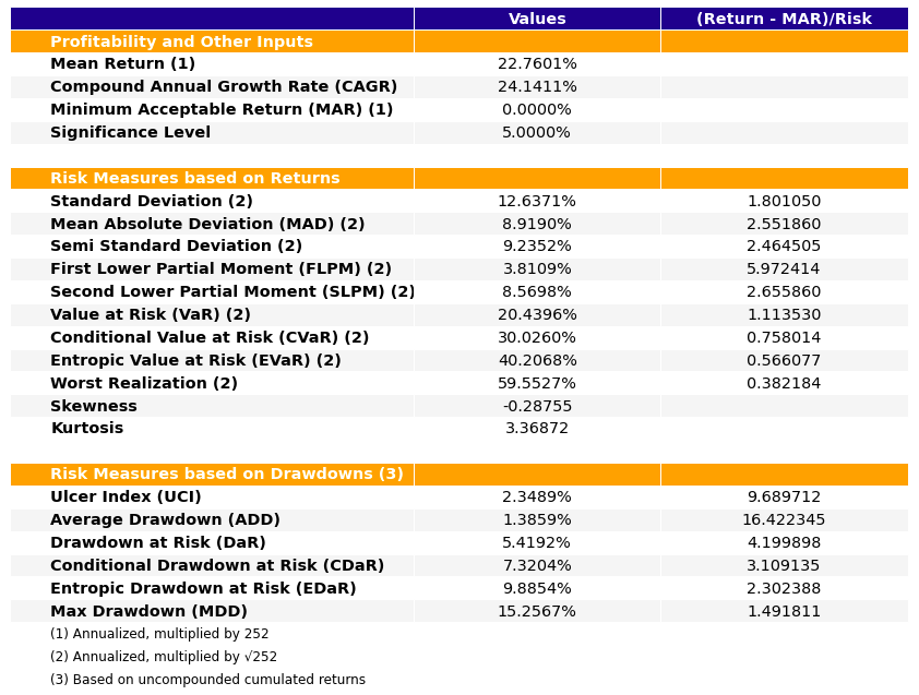

PlotFunctions.plot_clusters(returns, custom_cov=None, codependence='pearson', linkage='ward', opt_k_method='twodiff', k=None, max_k=10, bins_info='KN', alpha_tail=0.05, gs_threshold=0.5, leaf_order=True, show_clusters=True, dendrogram=True, cmap='RdYlBu', linecolor='fuchsia', title='', height=11, width=12, ax=None)[source]¶

Create a clustermap plot based on the selected codependence measure.

Parameters:¶

returns : DataFrame of shape (n_samples, n_assets)¶

Assets returns DataFrame, where n_samples is the number of observations and n_assets is the number of assets.

custom_cov : DataFrame or None, optional¶

Custom covariance matrix, used when codependence parameter has value ‘custom_cov’. The default is None.

codependence : str, can be {'pearson', 'spearman', 'abs_pearson', 'abs_spearman', 'distance', 'mutual_info', 'tail' or 'custom_cov'}¶

The codependence or similarity matrix used to build the distance metric and clusters. The default is ‘pearson’. Possible values are:

’pearson’: pearson correlation matrix. Distance formula: \(D_{i,j} = \sqrt{0.5(1-\rho_{i,j})}\).
’spearman’: spearman correlation matrix. Distance formula: \(D_{i,j} = \sqrt{0.5(1-\rho_{i,j})}\).
’kendall’: kendall correlation matrix. Distance formula: \(D_{i,j} = \sqrt{0.5(1-\rho^{kendall}_{i,j})}\).
’gerber1’: Gerber statistic 1 correlation matrix. Distance formula: \(D_{i,j} = \sqrt{0.5(1-\rho^{gerber1}_{i,j})}\).
’gerber2’: Gerber statistic 2 correlation matrix. Distance formula: \(D_{i,j} = \sqrt{0.5(1-\rho^{gerber2}_{i,j})}\).
’abs_pearson’: absolute value pearson correlation matrix. Distance formula: \(D_{i,j} = \sqrt{(1-|\rho_{i,j}|)}\).
’abs_spearman’: absolute value spearman correlation matrix. Distance formula: \(D_{i,j} = \sqrt{(1-|\rho_{i,j}|)}\).
’abs_kendall’: absolute value kendall correlation matrix. Distance formula: \(D_{i,j} = \sqrt{(1-|\rho^{kendall}_{i,j}|)}\).
’distance’: distance correlation matrix. Distance formula \(D_{i,j} = \sqrt{(1-|\rho_{i,j}|)}\).
’mutual_info’: mutual information matrix. Distance used is variation information matrix.
’tail’: lower tail dependence index matrix. Dissimilarity formula \(D_{i,j} = -\log{\lambda_{i,j}}\).
’custom_cov’: use custom correlation matrix based on the custom_cov parameter. Distance formula: \(D_{i,j} = \sqrt{0.5(1-\rho^{pearson}_{i,j})}\).

linkage : string, optional¶

Linkage method of hierarchical clustering, see linkage for more details. The default is ‘ward’. Possible values are:

’single’.
’complete’.
’average’.
’weighted’.
’centroid’.
’median’.
’ward’.
’DBHT’: Direct Bubble Hierarchical Tree.

opt_k_method : str¶

Method used to calculate the optimum number of clusters. The default is ‘twodiff’. Possible values are:

’twodiff’: two difference gap statistic.
’stdsil’: standarized silhouette score.

k : int, optional¶

Number of clusters. This value is took instead of the optimal number of clusters calculated with the two difference gap statistic. The default is None.

max_k : int, optional¶

Max number of clusters used by the two difference gap statistic to find the optimal number of clusters. The default is 10.

bins_info : int or str¶

Number of bins used to calculate variation of information. The default value is ‘KN’. Possible values are:

’KN’: Knuth’s choice method. See more in knuth_bin_width.
’FD’: Freedman–Diaconis’ choice method. See more in freedman_bin_width.
’SC’: Scotts’ choice method. See more in scott_bin_width.
’HGR’: Hacine-Gharbi and Ravier’ choice method.
int: integer value chosen by user.

alpha_tail : float, optional¶

Significance level for lower tail dependence index. The default is 0.05.

gs_threshold : float, optional¶

Gerber statistic threshold. The default is 0.5.

leaf_order : bool, optional¶

Indicates if the cluster are ordered so that the distance between successive leaves is minimal. The default is True.

show_clusters : bool, optional¶

Indicates if clusters are plot. The default is True.

dendrogram : bool, optional¶

Indicates if the plot has or not a dendrogram. The default is True.

cmap : str or cmap, optional¶

Colormap used to plot the pcolormesh plot. The default is ‘viridis’.

linecolor : str, optional¶

Color used to identify the clusters in the pcolormesh plot. The default is fuchsia’.

title : str, optional¶

Title of the chart. The default is “”.

height : float, optional¶

Height of the image in inches. The default is 12.

width : float, optional¶

Width of the image in inches. The default is 12.

ax : matplotlib axis, optional¶

If provided, plot on this axis. The default is None.

Raises:¶

ValueError – When the value cannot be calculated.

Returns:¶

ax – Returns the Axes object with the plot for further tweaking.

Return type:¶

matplotlib axis

Example

ax = rp.plot_clusters(returns=Y,
                      codependence='spearman',
                      linkage='ward',
                      k=None,
                      max_k=10,
                      leaf_order=True,
                      dendrogram=True,
                      ax=None)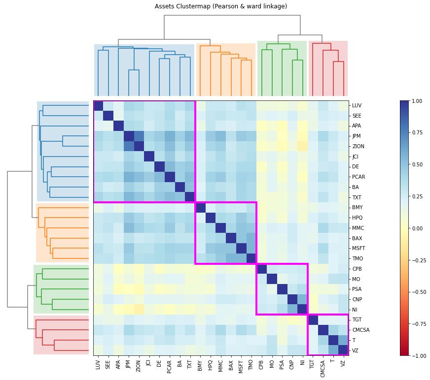

PlotFunctions.plot_dendrogram(returns, custom_cov=None, codependence='pearson', linkage='ward', opt_k_method='twodiff', k=None, max_k=10, bins_info='KN', alpha_tail=0.05, gs_threshold=0.5, leaf_order=True, show_clusters=True, title='', height=5, width=12, ax=None)[source]¶

Create a dendrogram based on the selected codependence measure.

Parameters:¶

returns : DataFrame of shape (n_samples, n_assets)¶

Assets returns DataFrame, where n_samples is the number of observations and n_assets is the number of assets.

custom_cov : DataFrame or None, optional¶

Custom covariance matrix, used when codependence parameter has value ‘custom_cov’. The default is None.

codependence : str, can be {'pearson', 'spearman', 'abs_pearson', 'abs_spearman', 'distance', 'mutual_info', 'tail' or 'custom_cov'}¶

The codependence or similarity matrix used to build the distance metric and clusters. The default is ‘pearson’. Possible values are:

’pearson’: pearson correlation matrix. Distance formula: \(D_{i,j} = \sqrt{0.5(1-\rho_{i,j})}\).
’spearman’: spearman correlation matrix. Distance formula: \(D_{i,j} = \sqrt{0.5(1-\rho_{i,j})}\).
’kendall’: kendall correlation matrix. Distance formula: \(D_{i,j} = \sqrt{0.5(1-\rho^{kendall}_{i,j})}\).
’gerber1’: Gerber statistic 1 correlation matrix. Distance formula: \(D_{i,j} = \sqrt{0.5(1-\rho^{gerber1}_{i,j})}\).
’gerber2’: Gerber statistic 2 correlation matrix. Distance formula: \(D_{i,j} = \sqrt{0.5(1-\rho^{gerber2}_{i,j})}\).
’abs_pearson’: absolute value pearson correlation matrix. Distance formula: \(D_{i,j} = \sqrt{(1-|\rho_{i,j}|)}\).
’abs_spearman’: absolute value spearman correlation matrix. Distance formula: \(D_{i,j} = \sqrt{(1-|\rho_{i,j}|)}\).
’abs_kendall’: absolute value kendall correlation matrix. Distance formula: \(D_{i,j} = \sqrt{(1-|\rho^{kendall}_{i,j}|)}\).
’distance’: distance correlation matrix. Distance formula \(D_{i,j} = \sqrt{(1-|\rho_{i,j}|)}\).
’mutual_info’: mutual information matrix. Distance used is variation information matrix.
’tail’: lower tail dependence index matrix. Dissimilarity formula \(D_{i,j} = -\log{\lambda_{i,j}}\).
’custom_cov’: use custom correlation matrix based on the custom_cov parameter. Distance formula: \(D_{i,j} = \sqrt{0.5(1-\rho^{pearson}_{i,j})}\).

linkage : string, optional¶

Linkage method of hierarchical clustering, see linkage for more details. The default is ‘ward’. Possible values are:

’single’.
’complete’.
’average’.
’weighted’.
’centroid’.
’median’.
’ward’.
’DBHT’: Direct Bubble Hierarchical Tree.

opt_k_method : str¶

Method used to calculate the optimum number of clusters. The default is ‘twodiff’. Possible values are:

’twodiff’: two difference gap statistic.
’stdsil’: standarized silhouette score.

k : int, optional¶

Number of clusters. This value is took instead of the optimal number of clusters calculated with the two difference gap statistic. The default is None.

max_k : int, optional¶

Max number of clusters used by the two difference gap statistic to find the optimal number of clusters. The default is 10.

bins_info : int or str¶

Number of bins used to calculate variation of information. The default value is ‘KN’. Possible values are:

’KN’: Knuth’s choice method. See more in knuth_bin_width.
’FD’: Freedman–Diaconis’ choice method. See more in freedman_bin_width.
’SC’: Scotts’ choice method. See more in scott_bin_width.
’HGR’: Hacine-Gharbi and Ravier’ choice method.
int: integer value chosen by user.

alpha_tail : float, optional¶

Significance level for lower tail dependence index. The default is 0.05.

gs_threshold : float, optional¶

Gerber statistic threshold. The default is 0.5.

leaf_order : bool, optional¶

Indicates if the cluster are ordered so that the distance between successive leaves is minimal. The default is True.

show_clusters : bool, optional¶

Indicates if clusters are plot. The default is True.

title : str, optional¶

Title of the chart. The default is “”.

height : float, optional¶

Height of the image in inches. The default is 5.

width : float, optional¶

Width of the image in inches. The default is 12.

ax : matplotlib axis, optional¶

If provided, plot on this axis. The default is None.

Raises:¶

ValueError – When the value cannot be calculated.

Returns:¶

ax – Returns the Axes object with the plot for further tweaking.

Return type:¶

matplotlib axis

Example

ax = rp.plot_dendrogram(returns=Y,
                        codependence='spearman',
                        linkage='ward',
                        k=None,
                        max_k=10,
                        leaf_order=True,
                        ax=None)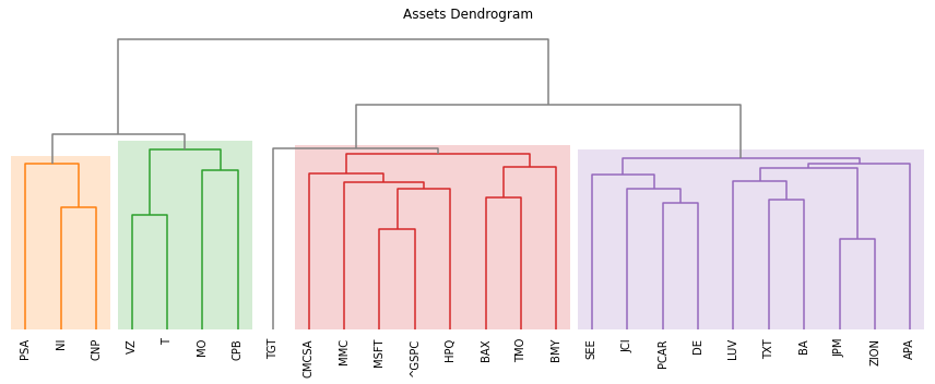

PlotFunctions.plot_network(returns, custom_cov=None, codependence='pearson', linkage='ward', opt_k_method='twodiff', k=None, max_k=10, bins_info='KN', alpha_tail=0.05, gs_threshold=0.5, leaf_order=True, kind='spring', seed=0, node_labels=True, node_size=1400, node_alpha=0.7, font_size=10, title='', height=8, width=10, ax=None)[source]¶

Create a network plot. The Planar Maximally Filtered Graph (PMFG) for DBHT linkage and Minimum Spanning Tree (MST) for other linkage methods.

Parameters:¶

returns : DataFrame of shape (n_samples, n_assets)¶

Assets returns DataFrame, where n_samples is the number of observations and n_assets is the number of assets.

custom_cov : DataFrame or None, optional¶

Custom covariance matrix, used when codependence parameter has value ‘custom_cov’. The default is None.

codependence : str, can be {'pearson', 'spearman', 'abs_pearson', 'abs_spearman', 'distance', 'mutual_info', 'tail' or 'custom_cov'}¶

The codependence or similarity matrix used to build the distance metric and clusters. The default is ‘pearson’. Possible values are:

’pearson’: pearson correlation matrix. Distance formula: \(D_{i,j} = \sqrt{0.5(1-\rho^{pearson}_{i,j})}\).
’spearman’: spearman correlation matrix. Distance formula: \(D_{i,j} = \sqrt{0.5(1-\rho^{spearman}_{i,j})}\).
’kendall’: kendall correlation matrix. Distance formula: \(D_{i,j} = \sqrt{0.5(1-\rho^{kendall}_{i,j})}\).
’gerber1’: Gerber statistic 1 correlation matrix. Distance formula: \(D_{i,j} = \sqrt{0.5(1-\rho^{gerber1}_{i,j})}\).
’gerber2’: Gerber statistic 2 correlation matrix. Distance formula: \(D_{i,j} = \sqrt{0.5(1-\rho^{gerber2}_{i,j})}\).
’abs_pearson’: absolute value pearson correlation matrix. Distance formula: \(D_{i,j} = \sqrt{(1-|\rho_{i,j}|)}\).
’abs_spearman’: absolute value spearman correlation matrix. Distance formula: \(D_{i,j} = \sqrt{(1-|\rho_{i,j}|)}\).
’abs_kendall’: absolute value kendall correlation matrix. Distance formula: \(D_{i,j} = \sqrt{(1-|\rho^{kendall}_{i,j}|)}\).
’distance’: distance correlation matrix. Distance formula \(D_{i,j} = \sqrt{(1-\rho^{distance}_{i,j})}\).
’mutual_info’: mutual information matrix. Distance used is variation information matrix.
’tail’: lower tail dependence index matrix. Dissimilarity formula \(D_{i,j} = -\log{\lambda_{i,j}}\).
’custom_cov’: use custom correlation matrix based on the custom_cov parameter. Distance formula: \(D_{i,j} = \sqrt{0.5(1-\rho^{pearson}_{i,j})}\).

linkage : string, optional¶

Linkage method of hierarchical clustering, see linkage for more details. The default is ‘ward’. Possible values are:

’single’.
’complete’.
’average’.
’weighted’.
’centroid’.
’median’.
’ward’.
’DBHT’: Direct Bubble Hierarchical Tree.

opt_k_method : str¶

Method used to calculate the optimum number of clusters. The default is ‘twodiff’. Possible values are:

’twodiff’: two difference gap statistic.
’stdsil’: standarized silhouette score.

k : int, optional¶

Number of clusters. This value is took instead of the optimal number of clusters calculated with the two difference gap statistic. The default is None.

max_k : int, optional¶

Max number of clusters used by the two difference gap statistic to find the optimal number of clusters. The default is 10.

bins_info : int or str¶

Number of bins used to calculate variation of information. The default value is ‘KN’. Possible values are:

’KN’: Knuth’s choice method. See more in knuth_bin_width.
’FD’: Freedman–Diaconis’ choice method. See more in freedman_bin_width.
’SC’: Scotts’ choice method. See more in scott_bin_width.
’HGR’: Hacine-Gharbi and Ravier’ choice method.
int: integer value chosen by user.

alpha_tail : float, optional¶

Significance level for lower tail dependence index. The default is 0.05.

gs_threshold : float, optional¶

Gerber statistic threshold. The default is 0.5.

leaf_order : bool, optional¶

Indicates if the cluster are ordered so that the distance between successive leaves is minimal. The default is True.

kind : str, optional¶

Kind of networkx layout. The default value is ‘spring’. Possible values are:

’spring’: networkx spring_layout.
’planar’. networkx planar_layout.
’circular’. networkx circular_layout.
’kamada’. networkx kamada_kawai_layout.

seed : int, optional¶

Seed for networkx spring layout. The default value is 0.

node_labels : bool, optional¶

Specify if node lables are visible. The default value is True.

node_size : float, optional¶

Size of the nodes. The default value is 1600.

node_alpha : float, optional¶

Alpha parameter or transparency of nodes. The default value is 0.7.

font_size : float, optional¶

Font size of node labels. The default value is 12.

title : str, optional¶

Title of the chart. The default is “”.

height : float, optional¶

Height of the image in inches. The default is 8.

width : float, optional¶

Width of the image in inches. The default is 10.

ax : matplotlib axis, optional¶

If provided, plot on this axis. The default is None.

Raises:¶

ValueError – When the value cannot be calculated.

Returns:¶

ax – Returns the Axes object with the plot for further tweaking.

Return type:¶

matplotlib axis

Example

ax = rp.plot_network(returns=Y,
                     codependence="pearson",
                     linkage="ward",
                     k=None,
                     max_k=10,
                     alpha_tail=0.05,
                     leaf_order=True,
                     kind='kamada',
                     ax=None)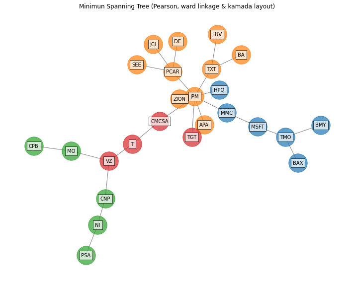

PlotFunctions.plot_network_allocation(returns, w, custom_cov=None, codependence='pearson', linkage='ward', bins_info='KN', alpha_tail=0.05, gs_threshold=0.5, leaf_order=True, kind='spring', seed=0, node_labels=True, max_node_size=2000, color_lng='tab:blue', color_sht='tab:red', label_v=0.08, label_h=0, font_size=10, title='', height=8, width=10, ax=None)[source]¶

Create a network plot with node size of the nodes and color represents the amount invested and direction (long-short) respectively. The Planar Maximally Filtered Graph (PMFG) for DBHT linkage and Minimum Spanning Tree (MST) for other linkage methods.

Parameters:¶

returns : DataFrame of shape (n_samples, n_assets)¶

Assets returns DataFrame, where n_samples is the number of observations and n_assets is the number of assets.

w : DataFrame or Series of shape (n_assets, 1)¶

Portfolio weights, where n_assets is the number of assets.

custom_cov : DataFrame or None, optional¶

Custom covariance matrix, used when codependence parameter has value ‘custom_cov’. The default is None.

codependence : str, can be {'pearson', 'spearman', 'abs_pearson', 'abs_spearman', 'distance', 'mutual_info', 'tail' or 'custom_cov'}¶

The codependence or similarity matrix used to build the distance metric and clusters. The default is ‘pearson’. Possible values are:

’pearson’: pearson correlation matrix. Distance formula: \(D_{i,j} = \sqrt{0.5(1-\rho^{pearson}_{i,j})}\).
’spearman’: spearman correlation matrix. Distance formula: \(D_{i,j} = \sqrt{0.5(1-\rho^{spearman}_{i,j})}\).
’kendall’: kendall correlation matrix. Distance formula: \(D_{i,j} = \sqrt{0.5(1-\rho^{kendall}_{i,j})}\).
’gerber1’: Gerber statistic 1 correlation matrix. Distance formula: \(D_{i,j} = \sqrt{0.5(1-\rho^{gerber1}_{i,j})}\).
’gerber2’: Gerber statistic 2 correlation matrix. Distance formula: \(D_{i,j} = \sqrt{0.5(1-\rho^{gerber2}_{i,j})}\).
’abs_pearson’: absolute value pearson correlation matrix. Distance formula: \(D_{i,j} = \sqrt{(1-|\rho_{i,j}|)}\).
’abs_spearman’: absolute value spearman correlation matrix. Distance formula: \(D_{i,j} = \sqrt{(1-|\rho_{i,j}|)}\).
’abs_kendall’: absolute value kendall correlation matrix. Distance formula: \(D_{i,j} = \sqrt{(1-|\rho^{kendall}_{i,j}|)}\).
’distance’: distance correlation matrix. Distance formula \(D_{i,j} = \sqrt{(1-\rho^{distance}_{i,j})}\).
’mutual_info’: mutual information matrix. Distance used is variation information matrix.
’tail’: lower tail dependence index matrix. Dissimilarity formula \(D_{i,j} = -\log{\lambda_{i,j}}\).
’custom_cov’: use custom correlation matrix based on the custom_cov parameter. Distance formula: \(D_{i,j} = \sqrt{0.5(1-\rho^{pearson}_{i,j})}\).

linkage : string, optional¶

Linkage method of hierarchical clustering, see linkage for more details. The default is ‘ward’. Possible values are:

’single’.
’complete’.
’average’.
’weighted’.
’centroid’.
’median’.
’ward’.
’DBHT’: Direct Bubble Hierarchical Tree.

bins_info : int or str¶

Number of bins used to calculate variation of information. The default value is ‘KN’. Possible values are:

’KN’: Knuth’s choice method. See more in knuth_bin_width.
’FD’: Freedman–Diaconis’ choice method. See more in freedman_bin_width.
’SC’: Scotts’ choice method. See more in scott_bin_width.
’HGR’: Hacine-Gharbi and Ravier’ choice method.
int: integer value chosen by user.

alpha_tail : float, optional¶

Significance level for lower tail dependence index. The default is 0.05.

gs_threshold : float, optional¶

Gerber statistic threshold. The default is 0.5.

leaf_order : bool, optional¶

Indicates if the cluster are ordered so that the distance between successive leaves is minimal. The default is True.

kind : str, optional¶

Kind of networkx layout. The default value is ‘spring’. Possible values are:

’spring’: networkx spring_layout.
’planar’. networkx planar_layout.
’circular’. networkx circular_layout.
’kamada’. networkx kamada_kawai_layout.

seed : int, optional¶

Seed for networkx spring layout. The default value is 0.

node_labels : bool, optional¶

Specify if node lables are visible. The default value is True.

max_node_size : float, optional¶

Size of the node with maximum weight in absolute value. The default value is 2000.

color_lng : str, optional¶

Color of assets with long positions. The default value is ‘tab:blue’.

color_sht : str, optional¶

Color of assets with short positions. The default value is ‘tab:red’.

label_v : float, optional¶

Vertical distance the label is offset from the center. The default value is 0.08.

label_h : float, optional¶

Horizontal distance the label is offset from the center. The default value is 0.

font_size : float, optional¶

Font size of node labels. The default value is 12.

title : str, optional¶

Title of the chart. The default is “”.

height : float, optional¶

Height of the image in inches. The default is 8.

width : float, optional¶

Width of the image in inches. The default is 10.

ax : matplotlib axis, optional¶

If provided, plot on this axis. The default is None.

Raises:¶

ValueError – When the value cannot be calculated.

Returns:¶

ax – Returns the Axes object with the plot for further tweaking.

Return type:¶

matplotlib axis

Example

ax = rp.plot_network_allocation(returns=Y,
                                w=w1,
                                codependence="pearson",
                                linkage="ward",
                                alpha_tail=0.05,
                                leaf_order=True,
                                kind='kamada',
                                ax=None)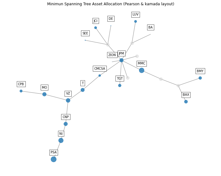

../_images/Assets_Network_Allocation.png

PlotFunctions.plot_clusters_network(returns, custom_cov=None, codependence='pearson', linkage='ward', opt_k_method='twodiff', k=None, max_k=10, bins_info='KN', alpha_tail=0.05, gs_threshold=0.5, leaf_order=True, seed=0, node_labels=True, node_size=2000, node_alpha=0.7, scale=10, subscale=5, font_size=10, title='', height=8, width=10, ax=None)[source]¶

Create a network plot that show each cluster obtained from the dendrogram as an independent graph.

Parameters:¶

returns : DataFrame of shape (n_samples, n_assets)¶

Assets returns DataFrame, where n_samples is the number of observations and n_assets is the number of assets.

custom_cov : DataFrame or None, optional¶

Custom covariance matrix, used when codependence parameter has value ‘custom_cov’. The default is None.

codependence : str, can be {'pearson', 'spearman', 'abs_pearson', 'abs_spearman', 'distance', 'mutual_info', 'tail' or 'custom_cov'}¶

The codependence or similarity matrix used to build the distance metric and clusters. The default is ‘pearson’. Possible values are:

’pearson’: pearson correlation matrix. Distance formula: \(D_{i,j} = \sqrt{0.5(1-\rho^{pearson}_{i,j})}\).
’spearman’: spearman correlation matrix. Distance formula: \(D_{i,j} = \sqrt{0.5(1-\rho^{spearman}_{i,j})}\).
’kendall’: kendall correlation matrix. Distance formula: \(D_{i,j} = \sqrt{0.5(1-\rho^{kendall}_{i,j})}\).
’gerber1’: Gerber statistic 1 correlation matrix. Distance formula: \(D_{i,j} = \sqrt{0.5(1-\rho^{gerber1}_{i,j})}\).
’gerber2’: Gerber statistic 2 correlation matrix. Distance formula: \(D_{i,j} = \sqrt{0.5(1-\rho^{gerber2}_{i,j})}\).
’abs_pearson’: absolute value pearson correlation matrix. Distance formula: \(D_{i,j} = \sqrt{(1-|\rho_{i,j}|)}\).
’abs_spearman’: absolute value spearman correlation matrix. Distance formula: \(D_{i,j} = \sqrt{(1-|\rho_{i,j}|)}\).
’abs_kendall’: absolute value kendall correlation matrix. Distance formula: \(D_{i,j} = \sqrt{(1-|\rho^{kendall}_{i,j}|)}\).
’distance’: distance correlation matrix. Distance formula \(D_{i,j} = \sqrt{(1-\rho^{distance}_{i,j})}\).
’mutual_info’: mutual information matrix. Distance used is variation information matrix.
’tail’: lower tail dependence index matrix. Dissimilarity formula \(D_{i,j} = -\log{\lambda_{i,j}}\).
’custom_cov’: use custom correlation matrix based on the custom_cov parameter. Distance formula: \(D_{i,j} = \sqrt{0.5(1-\rho^{pearson}_{i,j})}\).

linkage : string, optional¶

Linkage method of hierarchical clustering, see linkage for more details. The default is ‘ward’. Possible values are:

’single’.
’complete’.
’average’.
’weighted’.
’centroid’.
’median’.
’ward’.
’DBHT’: Direct Bubble Hierarchical Tree.

opt_k_method : str¶

Method used to calculate the optimum number of clusters. The default is ‘twodiff’. Possible values are:

’twodiff’: two difference gap statistic.
’stdsil’: standarized silhouette score.

k : int, optional¶

Number of clusters. This value is took instead of the optimal number of clusters calculated with the two difference gap statistic. The default is None.

max_k : int, optional¶

Max number of clusters used by the two difference gap statistic to find the optimal number of clusters. The default is 10.

bins_info : int or str¶

Number of bins used to calculate variation of information. The default value is ‘KN’. Possible values are:

’KN’: Knuth’s choice method. See more in knuth_bin_width.
’FD’: Freedman–Diaconis’ choice method. See more in freedman_bin_width.
’SC’: Scotts’ choice method. See more in scott_bin_width.
’HGR’: Hacine-Gharbi and Ravier’ choice method.
int: integer value chosen by user.

alpha_tail : float, optional¶

Significance level for lower tail dependence index. The default is 0.05.

gs_threshold : float, optional¶

Gerber statistic threshold. The default is 0.5.

leaf_order : bool, optional¶

Indicates if the cluster are ordered so that the distance between successive leaves is minimal. The default is True.

seed : int, optional¶

Seed for networkx spring layout. The default value is 0.

node_labels : bool, optional¶

Specify if node lables are visible. The default value is True.

node_size : float, optional¶

Size of the node. The default value is 2000.

node_alpha : float, optional¶

Alpha parameter or transparency of nodes. The default value is 0.7.

scale : float, optional¶

Scale of whole graph. The default value is 10.

subscale : float, optional¶

Scale of clusters. The default value is 5.

font_size : float, optional¶

Font size of node labels. The default value is 12.

title : str, optional¶

Title of the chart. The default is “”.

height : float, optional¶

Height of the image in inches. The default is 8.

width : float, optional¶

Width of the image in inches. The default is 10.

ax : matplotlib axis, optional¶

If provided, plot on this axis. The default is None.

Raises:¶

ValueError – When the value cannot be calculated.

Returns:¶

ax – Returns the Axes object with the plot for further tweaking.

Return type:¶

matplotlib axis

Example

ax = rp.plot_clusters_network(returns=Y,
                              codependence="pearson",
                              linkage="ward",
                              k=None,
                              max_k=10,
                              ax=None)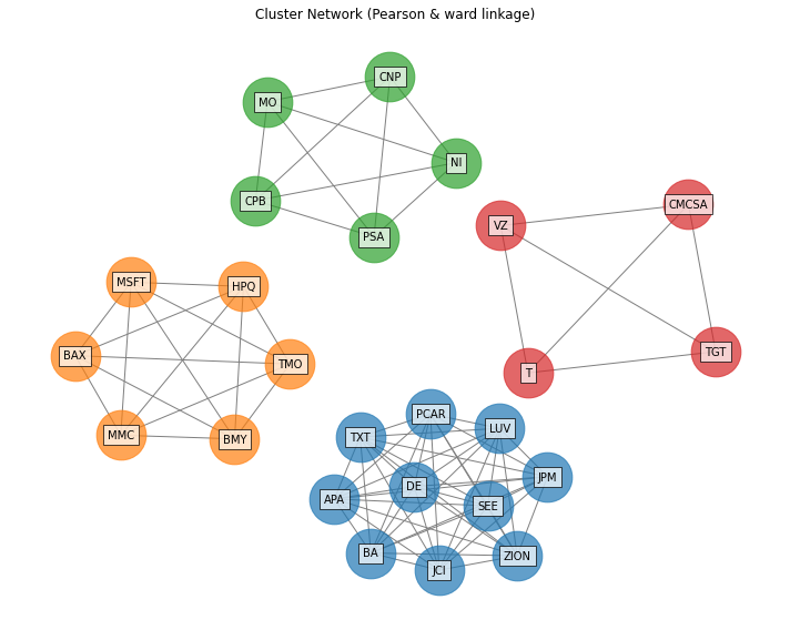

PlotFunctions.plot_clusters_network_allocation(returns, w, custom_cov=None, codependence='pearson', linkage='ward', opt_k_method='twodiff', k=None, max_k=10, bins_info='KN', alpha_tail=0.05, gs_threshold=0.5, leaf_order=True, seed=0, node_labels=True, max_node_size=2000, color_lng='tab:blue', color_sht='tab:red', scale=10, subscale=5, label_v=1.5, label_h=0, font_size=10, title='', height=8, width=10, ax=None)[source]¶

Create a network plot that show each cluster obtained from the dendrogram as an independent graph. The size of the nodes and color represents the amount invested and direction (long-short) respectively.

Parameters:¶

returns : DataFrame of shape (n_samples, n_assets)¶

Assets returns DataFrame, where n_samples is the number of observations and n_assets is the number of assets.

w : DataFrame or Series of shape (n_assets, 1)¶

Portfolio weights, where n_assets is the number of assets.

custom_cov : DataFrame or None, optional¶

Custom covariance matrix, used when codependence parameter has value ‘custom_cov’. The default is None.

codependence : str, can be {'pearson', 'spearman', 'abs_pearson', 'abs_spearman', 'distance', 'mutual_info', 'tail' or 'custom_cov'}¶

The codependence or similarity matrix used to build the distance metric and clusters. The default is ‘pearson’. Possible values are:

’pearson’: pearson correlation matrix. Distance formula: \(D_{i,j} = \sqrt{0.5(1-\rho^{pearson}_{i,j})}\).
’spearman’: spearman correlation matrix. Distance formula: \(D_{i,j} = \sqrt{0.5(1-\rho^{spearman}_{i,j})}\).
’kendall’: kendall correlation matrix. Distance formula: \(D_{i,j} = \sqrt{0.5(1-\rho^{kendall}_{i,j})}\).
’gerber1’: Gerber statistic 1 correlation matrix. Distance formula: \(D_{i,j} = \sqrt{0.5(1-\rho^{gerber1}_{i,j})}\).
’gerber2’: Gerber statistic 2 correlation matrix. Distance formula: \(D_{i,j} = \sqrt{0.5(1-\rho^{gerber2}_{i,j})}\).
’abs_pearson’: absolute value pearson correlation matrix. Distance formula: \(D_{i,j} = \sqrt{(1-|\rho_{i,j}|)}\).
’abs_spearman’: absolute value spearman correlation matrix. Distance formula: \(D_{i,j} = \sqrt{(1-|\rho_{i,j}|)}\).
’abs_kendall’: absolute value kendall correlation matrix. Distance formula: \(D_{i,j} = \sqrt{(1-|\rho^{kendall}_{i,j}|)}\).
’distance’: distance correlation matrix. Distance formula \(D_{i,j} = \sqrt{(1-\rho^{distance}_{i,j})}\).
’mutual_info’: mutual information matrix. Distance used is variation information matrix.
’tail’: lower tail dependence index matrix. Dissimilarity formula \(D_{i,j} = -\log{\lambda_{i,j}}\).
’custom_cov’: use custom correlation matrix based on the custom_cov parameter. Distance formula: \(D_{i,j} = \sqrt{0.5(1-\rho^{pearson}_{i,j})}\).

linkage : string, optional¶

Linkage method of hierarchical clustering, see linkage for more details. The default is ‘ward’. Possible values are:

’single’.
’complete’.
’average’.
’weighted’.
’centroid’.
’median’.
’ward’.
’DBHT’: Direct Bubble Hierarchical Tree.

bins_info : int or str¶

Number of bins used to calculate variation of information. The default value is ‘KN’. Possible values are:

’KN’: Knuth’s choice method. See more in knuth_bin_width.
’FD’: Freedman–Diaconis’ choice method. See more in freedman_bin_width.
’SC’: Scotts’ choice method. See more in scott_bin_width.
’HGR’: Hacine-Gharbi and Ravier’ choice method.
int: integer value chosen by user.

alpha_tail : float, optional¶

Significance level for lower tail dependence index. The default is 0.05.

gs_threshold : float, optional¶

Gerber statistic threshold. The default is 0.5.

leaf_order : bool, optional¶

Indicates if the cluster are ordered so that the distance between successive leaves is minimal. The default is True.

seed : int, optional¶

Seed for networkx spring layout. The default value is 0.

node_labels : bool, optional¶

Specify if node lables are visible. The default value is True.

max_node_size : float, optional¶

Size of the node with maximum weight in absolute value. The default value is 2000.

color_lng : str, optional¶

Color of assets with long positions. The default value is ‘tab:blue’.

color_sht : str, optional¶

Color of assets with short positions. The default value is ‘tab:red’.

scale : float, optional¶

Scale of whole graph. The default value is 10.

subscale : float, optional¶

Scale of clusters. The default value is 5.

label_v : float, optional¶

Vertical distance the label is offset from the center. The default value is 1.5.

label_h : float, optional¶

Horizontal distance the label is offset from the center. The default value is 0.

font_size : float, optional¶

Font size of node labels. The default value is 10.

title : str, optional¶

Title of the chart. The default is “”.

height : float, optional¶

Height of the image in inches. The default is 8.

width : float, optional¶

Width of the image in inches. The default is 10.

ax : matplotlib axis, optional¶

If provided, plot on this axis. The default is None.

Raises:¶

ValueError – When the value cannot be calculated.

Returns:¶

ax – Returns the Axes object with the plot for further tweaking.

Return type:¶

matplotlib axis

Example

ax = rp.plot_clusters_network_allocation(returns=Y,
                                         w=w1,
                                         codependence="pearson",
                                         linkage="ward",
                                         k=None,
                                         max_k=10,
                                         ax=None)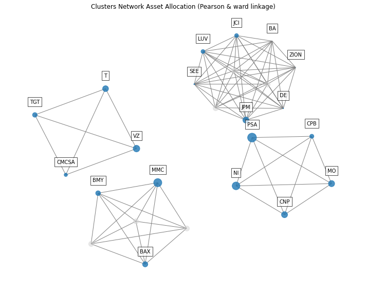

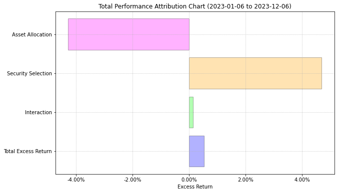
../_images/Assets_Clusters_Network_Allocation.png

PlotFunctions.plot_BrinsonAttribution(prices, w, wb, start, end, asset_classes, classes_col, method='nearest', sector='Total', height=6, width=10, ax=None)[source]¶

Creates a plot with the Brinson Performance Attribution specified by the sector parameter.

Parameters:¶

prices : DataFrame of shape (n_samples, n_assets)¶: Assets prices DataFrame, where n_samples is the number of observations and n_assets is the number of assets.
w : DataFrame or Series of shape (n_assets, 1)¶: A portfolio specified by the user.
wb : DataFrame or Series of shape (n_assets, 1)¶: A benchmark specified by the user.
start : str¶: Start date in format ‘YYYY-MM-DD’ specified by the user.
end : str¶: End date in format ‘YYYY-MM-DD’ specified by the user.
asset_classes : DataFrame of shape (n_assets, n_cols)¶: Asset’s classes DataFrame, where n_assets is the number of assets and n_cols is the number of columns of the DataFrame where the first column is the asset list and the next columns are the different asset’s classes sets. It is only used when kind value is ‘classes’. The default value is None.
classes_col : str or int¶: If value is str, it is the column name of the set of classes from asset_classes dataframe. If value is int, it is the column number of the set of classes from asset_classes dataframe. The default value is None.
method : str¶: Method used to calculate the nearest start or end dates in case one of them is not in prices DataFrame. The default value is ‘nearest’. See get_indexer for more details.
sector : str¶: Is the sector or class for which the function will plot the Brinson performance attribution. Possible values are all classes in the set of classes specified by classes_col parameter and ‘Total’ for aggregate performance attribution. Default value is ‘Total’.
height : float, optional¶: Height of the image in inches. The default is 8.
width : float, optional¶: Width of the image in inches. The default is 10.
ax : matplotlib axis, optional¶: If provided, plot on this axis. The default is None.

Raises:¶

ValueError – When the value cannot be calculated.

Returns:¶

ax – Returns the Axes object with the plot for further tweaking.

Return type:¶

matplotlib axis.

Example

ax = plot_BrinsonAttribution(
    prices=data,
    w=w,
    wb=wb,
    start='2019-01-07',
    end='2019-12-06',
    asset_classes=asset_classes,
    classes_col='Industry',
    method='nearest',
    sector='Total',
    height=6,
    width=10,
    ax=None
    )